Speech signal representations

Feb 01, 2014

One of the objectives of our project is to learn a useful representation from speech signals that can be used to synthesize new (arbitrary) sentences. There are many different ways of representing speech signals; those representations are usually tailored to specific applications. In speech recognition, for example, we want to minimize the variability from different speakers while keeping sufficient information to discriminate different phonemes. In speech coding, however, we usually want to keep information that is associated with the speaker's identity as well as reduce the amount of data to be stored/transmitted.

Our dataset was initially distributed as frame MFCCs (input) and one-hot encoded phonemes (labels). While this representation is usually enough for speech recognition, I believe it is not enough for learning a useful representation for synthesis (as briefly mentioned by Laurent Dinh in his post). The reason is that MFCCs are a destructive/lossy representation of a speech signal. First, fundamental frequency information is completely lost, as well as instantaneous phase. MFCCs more or less represent the energy in different frequency channels that are considered important for human speech (following the Mel scale [Stevens2005]).

In this post, I will present some alternative speech signal representations that may be more suitable for speech synthesis. Even though one of our objectives is to learn a representation, we need to understand a little bit about what has been developed by the speech processing community, as it can serve as an inspiration.

Acoustic samples (time domain)

Using raw acoustic samples from overlapping frames is the simplest approach. A discrete signal \(x[n]\) is simply a sequence of (real or integer) numbers corresponding to the signal samples (sampled uniformly at an arbitrary sampling rate). The usual sampling rate for speech recognition applications is 16 kHz, while the sampling rate used for "telephone speech" coding is 8 kHz. This is essentially the information we find in a PCM-encoded WAV file.

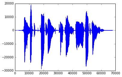
Time-domain speech signal sampled at 16 kHz.

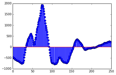
Zoom of a 200-sample segment of the above signal.

Short-time Fourier Transform

Another possible representation is to use Short-time Fourier Transform (STFT) coefficients from overlapping frames. This is essentially the same as using raw acoustic samples in the sense that there is no information loss, but the representation in the frequency domain is usually clearer for humans because we can associate the content in different frequency bands with different phonemes. The STFT of a discrete signal \(x[n]\) is given by:

\begin{equation*} STFT{x[n]}(m,\omega) = X(m,\omega) = \sum_{n=-\infty}^{\infty} x[n] w[n-m] e^{-j \omega n} \end{equation*}

where \(n,\omega\) are the time and frequency indexes, and \(w[n]\) is the windowing function. A spectrogram is the magnitude-squared version of this equation (i.e., without phase information).

Spectrograms can be done using windows with different lengths. This is related to the Gabor (or Heisenberg-Gabor) limit: we cannot simultaneously localize a signal in both time and frequency domains with a high degree of certainty. Therefore, we usually have to use different window lengths depending on what we want to analyze: wide windows have better frequency resolution and bad time resolution, while the opposite happens for short windows. A possible compromise is to choose a single window length that has sufficient resolution for the target application.

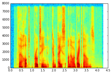
Spectrogram (using a 20 ms rectangular window) of the speech signal above.

Linear Predictive Coding

Linear Predictive Coding [o1988linear] coefficients + residual (basically excitation information). LPC is based on the source-filter model of speech production, which assumes a speech signal is produced by filtering a series of pulses (and eventually noise bursts). The LPC coefficients are related to the position of the articulators in the mouth (e.g., tongue, palate, lips), while the pitch/noise information is related to how the vocal tract is excited. This is usually represented as an auto-regressive (AR) model with order \(p\):

\begin{equation*} x[n] = \sum_{k=1}^{p} a_k x[n-k] \end{equation*}

where \(a[k]\) are the model's coefficients. LPCs are computed for each speech frame based on a least-squares method:

\begin{equation*} \arg\min_{a_k} \sum_{-\infty}^\infty [x[n] - \sum_{k=1}^p a_k x[n-k]]^2 \end{equation*}

Because of its error criteria, LPC also has problems to represent the phase of acoustic signals (by squaring the error, we are modeling the spectral magnitude of the signal, and not the phase). For this reason, LPC speech may sound artificial when resynthesized. More robust methods are used nowadays, such as the code-excited linear prediction (CELP) [valin2006speex]. These methods, for example, use psychoacoustics-inspired techniques to shape the coding noise to frequency regions where the human auditory system is more tolerant. In CELP, the residual is not transmitted directly, but represented as entries in two codebooks.

Wavelets

Them main purpose of a wavelet transform is to decompose arbitrary signals into localized contributions that can be labelled by a scale (or resolution) parameter [mallat1989theory]. The representation achieved through the wavelet transform can be seen as hierarchical: at a coarse resolution, we have an idea of “context”, while with highest resolution we can see more details. This is achieved by decomposing the original signal using a set of functions well-localized both in time and frequency (the so-called wavelets).

Discrete wavelet transforms are implemented as a cascade of digital filters with transfer functions derived from a discrete "mother wavelet". The figure below shows an example. Check also the notebook for an example of wavelet decomposition of the audio signal shown above.

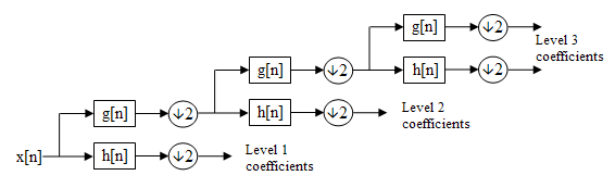
Filter bank used by a discrete wavelet transform with 3 levels of decomposition (image from the WikiMedia Commons ).

Sparse coding and dictionary-based methods

Sparse signal approximations are the basis for a variety of signal processing techniques. Such approximations are usually employed with the objective of having a signal representation that is more meaningful, malleable, and robust to noise than the ones obtained by standard transform methods [Sturm]. The so-called dictionary-based methods (DBM) decompose a signal into a linear combination of waveforms through an approximation technique such as Matching Pursuit (MP) [Mallat1993] or Orthogonal Matching Pursuit (OMP) [Pati1993]. The collection of waveforms that can be selected for the linear combination is called a dictionary. This dictionary is usually overcomplete, either because it is formed by merging complete dictionaries or because the functions are chosen arbitrarily.

I will talk more about sparse coding and dictionary-based methods later, since sparse coding is one of the methods we'll see in the course.

IPython notebook

An IPython notebook with examples for all the representations described here (except sparse coding) is available on my GitHub repo. You will need to install the packages PyWavelets and scikits.talkbox (both are available at PyPI) to be able to run it. If you just want to take a look without interacting with the code, you can access it here.

References

[Stevens2005]

S. S. Stevens, J. Volkmann, and E. B. Newman, “A Scale for the Measurement of the Psychological Magnitude Pitch,” The Journal of the Acoustical Society of America, vol. 8, no. 3, pp. 185–190, Jun. 2005.

[o1988linear]

D. O’Shaughnessy, “Linear predictive coding,” IEEE Potentials, vol. 7, no. 1, pp. 29–32, Feb. 1988.

[valin2006speex]

J.-M. Valin, “Speex: a free codec for free speech,” in Australian National Linux Conference, Dunedin, New Zealand, 2006.

[mallat1989theory]

S. G. Mallat, “A theory for multiresolution signal decomposition: the wavelet representation,” Pattern Analysis and Machine Intelligence, IEEE Transactions on, vol. 11, no. 7, pp. 674–693, 1989.

[Sturm]

B. L. Sturm, C. Roads, A. McLeran, and J. J. Shynk, “Analysis, Visualization, and Transformation of Audio Signals Using Dictionary-based Methods†,” Journal of New Music Research, vol. 38, no. 4, pp. 325–341, 2009.

[Mallat1993]

S. G. Mallat and Z. Zhang, “Matching pursuits with time-frequency dictionaries,” IEEE Transactions on Signal Processing, vol. 41, no. 12, pp. 3397–3415, Dec. 1993.

[Pati1993]

Y. C. Pati, R. Rezaiifar, and P. S. Krishnaprasad, “Orthogonal matching pursuit: Recursive function approximation with applications to wavelet decomposition,” in Signals, Systems and Computers, 1993. 1993 Conference Record of The Twenty-Seventh Asilomar Conference on, 1993, pp. 40–44.

This entry was tagged as ift6266