Using an auditory-inspired representation for speech
Mar 31, 2014
I previously described an approach to representing speech signals by decomposing them to an arbitrary dictionary (using a sparse coding algorithm such as Orthogonal Matching Pursuit). In that post, I showed that learning a representation from the data by using a dictionary learning method could be useful. However, there were some problems with that approach. First, the dictionary atoms were not localized in time: the atoms I learned from the data were waveforms spreading throughout the entire frame. This behavior has led to issues when reconstructing the signal, as nothing guarantees the last sample in the \(k^{th}\) frame will be close to the first sample in the \(k+1^{th}\) frame. The second issue was related to not using overlapped windows to split/resynthesize the signal. This is one of the main reasons that made the signals I generated previously so noisy.
In order to solve these problems, I added two updates to my previous code:
- Dropped the dictionary I learned from the data and switched to a gammatone dictionary.
- Generated the audio frames using Hamming windows with 50% overlap.
In the next sections, I will give a brief description and motivation for each of these updates. I will also show why they didn't work as well as I expected and inspired another architecture.
Gammatone functions and gammatone-based dictionary
Gammatone filters are a popular way of modeling the auditory processing at the cochlea. Basically, the cochlea is interpreted as a filterbank whose impulse response follows the following equation (the product of a gamma function and a cosine, or a pure tone):
In this equation, \(b\) corresponds to the filter's bandwidth, \(n\) is the filter order, \(f\) is the central frequency, and \(\phi\) is the phase of the carrier. The first two parameters can be fixed for the entire filterbank, while the center frequencies \(f\) are usually defined according to the cochlea's critical frequencies. One way of computing these frequencies is by using the Equivalent Rectangular Bandwidth (ERB), which gives an approximation to the bandwidths of the human auditory filters:
Here, \(Q_{ear} = 9.26449\) and \(B_{min} = 24.7\) are constants corresponding to the Q factor and minimum bandwidth of human auditory filters.
Gammatone functions are used in auditory modelling because they match the resonance of different regions in the cochlea. As shown in [Smith2006], human speech can be sparsely represented by gammatone atoms. [Strahl2008] has later shown that a sparse gammatone model can be optimized for English speech, even though the optimized model does not match the human auditory filters anymore.
A gammatone dictionary can be built similarly to a Gabor dictionary, as gammatones are localized both in time and frequency. First, we have to choose a set of frequencies; usually, you pick the number of frequencies you want and the range, and use the ERB equation to find equally-spaced frequencies in the ERB space (these would be the so called critical frequencies). Then, we select the resolution of our atoms (which has to be less or equal to the frame length in our application) and then time-shift the atoms inside the frame by a specified amount. The following Python code does that (and also normalizes the dictionary at the end):
def gammatone_matrix(b, fc, resolution, step):
    """Dictionary of gammatone functions"""
     centers = np.arange(0, resolution - step, step)
     D = np.empty((len(centers), resolution))
     for i, center in enumerate(centers):
         D[i] = gammatone_function(resolution, fc, center, b=b)
     D /= np.sqrt(np.sum(D ** 2, axis=1))[:, np.newaxis]
     return D
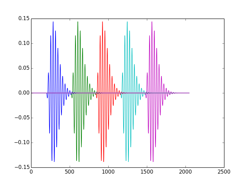
For illustration, see below 5 time-shifted versions of the same gammatone (note that in the actual dictionary, we probably want the time-shifted atoms to overlap a bit more than in this figure).
See my gammatone sparse coding library here, and an updated version of my IPython notebook for sparse coding there for more details. The test code in the library reads a wave file, segments it in 2048 frames with 50% overlap, windows each frame with a Hanning window (see next section for details) and decomposes each frame using gammatone atoms. The reconstruction in this example uses 200 non-zero coefficients per frame and the dictionary has 3150 atoms. This amounts for a compression of more than 10 times, but the reconstruction does not sound as bad as the ones we've seen previously.
Overlapping windows
A window function is a function that has non-zero values only inside a given interval. The most classical example of it is the rectangular window:
However, a problem with the rectangular window is that it does nothing to smooth the signal at the window borders. If we are processing a signal on a per-frame basis and then reconstructing it by concatenating the processed frames, nothing guarantees continuity when we join the processed frames. These abrupt changes introduce broadband noise bursts in our signal, which is something that we probably do not want!
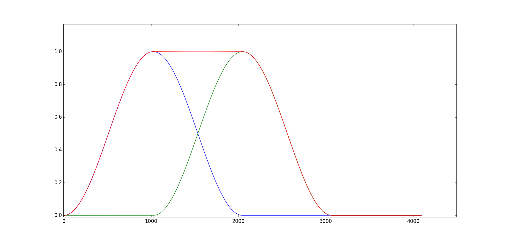
A way to mitigate this problem is to do overlap-add synthesis. Instead of shifting a full frame at a time and using rectangular windows, we overlap frames by a certain amount (25%, 50%, and 75% are often used values) and multiply each frame by a smooth window. We use window functions in such a way that the overlapped windows always sum to unity. The figure below shows two Hamming windows with an overlap of 50% (blue and green curves), and the sum of both windows (red curve). If we keep overlapping windows like this, overlap-add is an identity operation (i.e., we do not change the final result as long as we do not process the frames). Of course, in our case we are processing the frames, but overlap-add will help a bit in mitigating the abrupt changes between frames as we are now summing the values in overlapping frames to reconstruct our output instead of just connecting two non-overlapping frames.
Experiment with sparse coding using gammatone atoms
Based on the ideas described above, I generated a sparse-coded version of the TIMIT dataset using my gammatone sparse coding library. I used gammatones with 50 different cosine frequencies between 150 and 8000 Hz, timeshifts of 8 samples, and frames of length 160 with 50% overlap. For each frame, a sparse representation using 16 non-zero coefficients was extracted by using Orthogonal Matching Pursuit with a sparsity constraint.
This data and the one-hot encoded information about the previous, current, and next phone were used to train an MLP with the following characteristics:
- Two rectified linear hidden layers (2150 and 950 units, respectively);
- Linear output layer with 950 units (one for each sparse coding coefficient);
- Training: batch gradient descent (batch size of 512 samples), with squared error objective;
- Termination criteria: 10 epochs with objective decrease lower than \(10^{-6}\) or 200 epochs.
However, something strange happened when I tried to train this network: it has converged after 10 epochs! Of course this would be too good to be true, which means something terrible happened instead. In my case, the training, testing, and validation objectives did not change at all with training iterations. I still do not know exactly what happened, but I suspect the large amount of zeros in the input and target values made the majority of the gradients equal to zero, and without gradients none of the weights will change. Maybe a different kind of initialization could solve this issue, but there are other problems as well. Namely, this network does nothing to enforce sparsity at the output, and in the end the output coefficients will have a distribution that is very different from the target coefficients (which are zero most of the time). Prof. Bengio suggested that I could try making the output distribution the product of a Bernoulli distribution and a Gaussian distribution: the first one would say if that coefficient should be zero or not, and the latter would give its value. However, he noted that this is just an arbitrary statistical model which probably does not correspond to the real behavior of the coefficients, and we would probably be better by trying to estimate this distribution too (maybe with an RBM).
While trying to solve these issues, I had an idea for another architecture that could be easier to implement...
Splitting signal into spectral envelope and phase
As Jessica pointed out in her blog, most of the relevant information in a speech signal is encoded in its envelope. Because of that, we are less sensitive to phase distortions than to envelope distortions. As we have already discussed in class, as speech envelope variations are slower than the phase variations, some speech coding models (such as LPC) take these facts into account by encoding the envelope and the phase separately (and usually using a simpler model for the phase than for envelopes).
It was also brought to my attention that a recent paper [Han2014] to be presented at this year's ICASSP uses gammatone filterbank features to find spectral masks to use in speech dereverberation. The advantage of using gammatone filterbanks instead of a simple STFT is that with the gammatone filterbank, we are able to fine-tune spectral resolution at lower frequency bands (the most important band for speech content). While speech dereverberation is a totally different topic, the feature space used in that paper is still relevant. They are looking for spectral masks to filter an existing signal and not on synthesis, so they can discard the phase completely. For our project, we cannot do that but we could work with a slightly different approach.
We have one network that is trained on spectral envelopes, using a similar approach to that of the paper. This network is trained using the gammatonegram, which consists of the total gammatone band energy in all channels of our filterbank per frame. The figure below depicts how this is done:
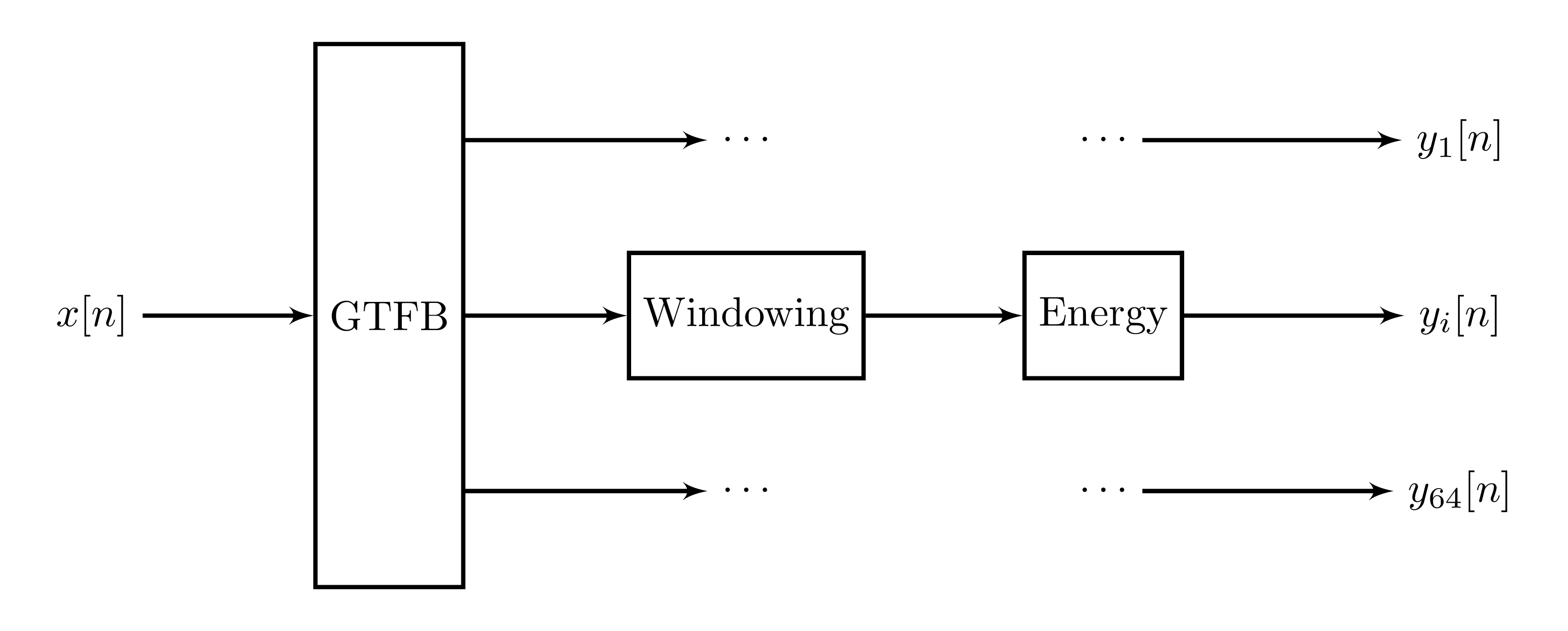
Here, \(y_i[n], i = 1, \dots, 64\) are the frame energies (sum of squared samples) for each gammatone channel (I'm using 64 channels here as this is what was used in [Han2014] and can be a good starting point). As inputs of this network, we would use the gammatonegram of a number of previous frames, one-hot encoded phones for these frames (and possibly some of the next frames), and the output would be the gammatonegram of the next frame. This is not enough to resynthesize a speech signal as we don't have the phase, but that could be solved by training a separate model for phases, either for an overall phase or a per-channel phase. Resynthesis is done according to the following signal flow diagram:
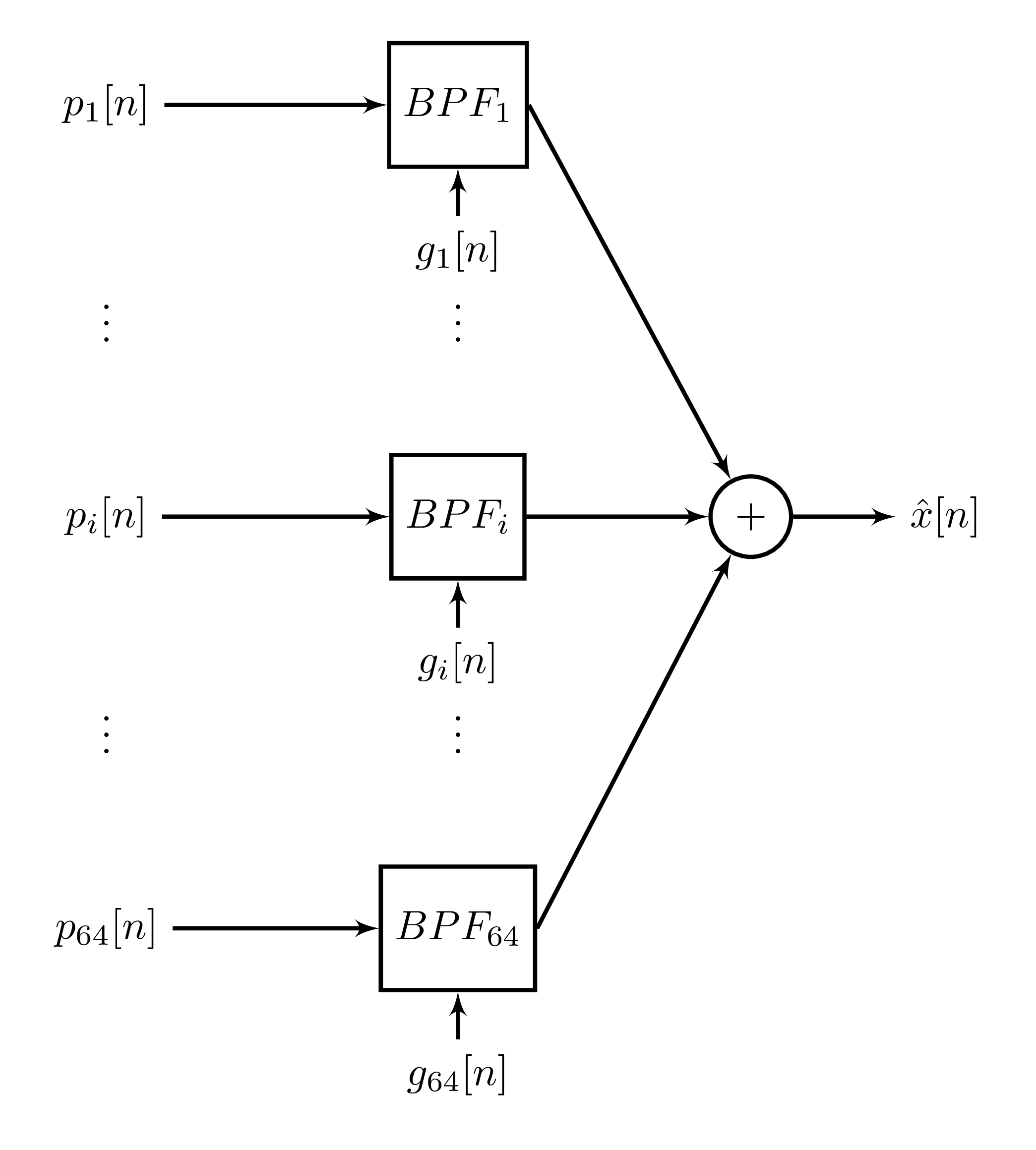
Here, \(p_i[n], i=1, \dots, 64\) are vectors representing the phase of each channel and \(g_i[n], i=1, \dots, 64\) are the amplitudes for each gammatone channel (which could be either the \(y_i[n]\) values computed before for each frame or a smoothed version of them).
For the network architecture, I am planning on using an MLP (possibly with unsupervised pretraining) for the spectral envelopes. For the phase components, I will initially try RBMs using previous phase samples, phone codes, and speaker characteristics (pitch, gender, etc.) as input. I expect to be able to use simpler models for the phase (or at least be able to control this model's complexity, as I believe there should be a tradeoff between speech quality and the accuracy of the phase models). I have already extracted the gammatone features from the whole database and will report results for the spectral envelope model on my next post.
References
| [Smith2006] | E. C. Smith and M. S. Lewicki, “Efficient auditory coding,” Nature, vol. 439, no. 7079, pp. 978–982, 2006. |
| [Strahl2008] | S. Strahl and A. Mertins, “Sparse gammatone signal model optimized for English speech does not match the human auditory filters,” Brain research, vol. 1220, pp. 224–233, 2008. |
| [Han2014] | (1, 2) K. Han, Y. Wang and D. Wang, “Learning spectral mapping for speech dereverberation”, To appear in the Proceedings of the IEEE ICASSP 2014, 2014. Available at http://www.cse.ohio-state.edu/~dwang/papers/HWW.icassp14.pdf. |